[cs231n] Summary
cs231n: Summary
Neural Networks
Image Classification: Data-driven Approach, k-Nearest Neighbor, train/val/test splits
Image Classification
Using a set of labeled images to predict categories of a set of test images. Then we can measure the accuracy of the predictions.
Nearest Neighbor classifier
- Choose a distance(L1, L2, etc.)
- Calculate the sum of the distance between each text data and all the train data. Get the closest one. The label of this data is what the classifier predict.
kNN classifier
Find the top k closest images and then have them vote on the label of the test image.
Validation set, cross-validation
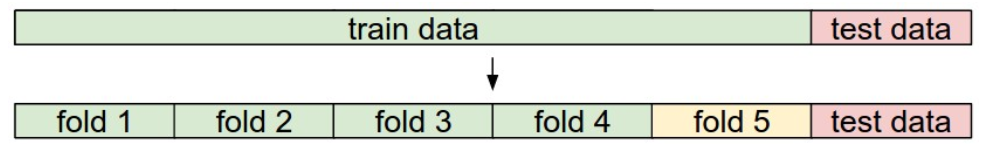
In this picture, fold 5 is the validation set. For cross-validation, we let fold 1-5 be validation set separately to help us choose some hyperparameters.
Linear classification: Support Vector Machine, Softmax
What we want: a map from images to label scores. \(\Rightarrow\) Score function, Loss function
Score function
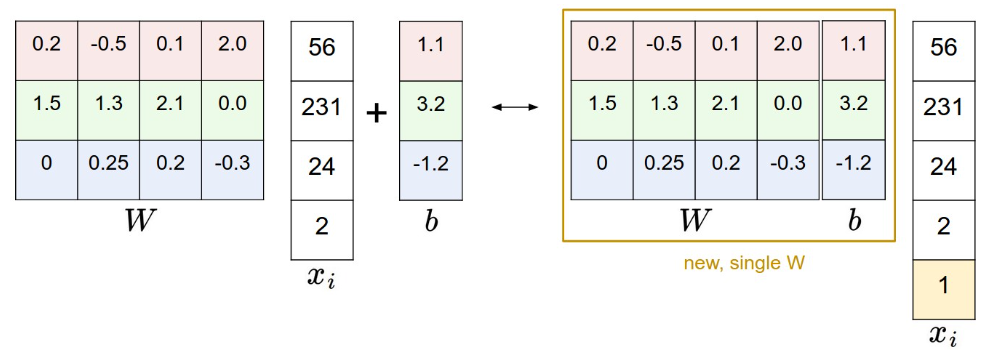
\(x_i\) is a picture and \(W\) is a matrix named weights. And \(b\) is bias.
\[
f(x_i,W,b)=Wx_i+b
\] Sometimes we can extend \(W\):
Preprocessing: center the data
For photos, pixel value: [0~255]
Now: [0…255] \(\Rightarrow\) [-127 .. 127] \(\Rightarrow\) [-1,1]
Loss function
Multiclass Support Vector Machine loss
For image \(x_i\) with label \(y_i\). Score function is \(f(x_i,W)\). Let \(s_j = f(x_i,W)_j\). Multiclass SVM loss: \[ L_i = \sum_{j\neq y_i}max(0,s_j-s_{y_i}+\Delta) \]
Regularization
\[ R(W) = \sum_k\sum_l W_{k,l}^2\\ L=\frac{1}{N}\sum_i L_i + \lambda R(W) \]
Or \[ L=\frac{1}{N}\sum_i\sum_{j\neq y_i}[max(0,f(x_i,W))_j-f(x_i,W)_{y_i}+\Delta]+\lambda \sum_k\sum_lW_{k,l}^2 \]
Softmax classifier
With \(f(x_i,W)=Wx_i\) unchanged, but for the loss: \[ L_i=-log(\frac{e^{f_{y_i}}}{\sum_je^{f_j}})\;or\;L_i=-f_{y_i}+log\sum_je^{f_j} \]
Optimization: Stochastic Gradient Descent
Visualizing the loss function
Optimization
Random search
Random local search
Following the gradient
\[ \frac{df(x)}{dx}=\lim_{h\rightarrow 0}\frac{f(x+h)-f(x)}{h} \]
Use this definition to calculate grad of all dims
1 | |
In fact, we usually use \[ \frac{f(x+h)-f(x-h)}{2h} \] But this method of calculation is expensive and not so accurate. So maybe we can do it in a more “math” way.
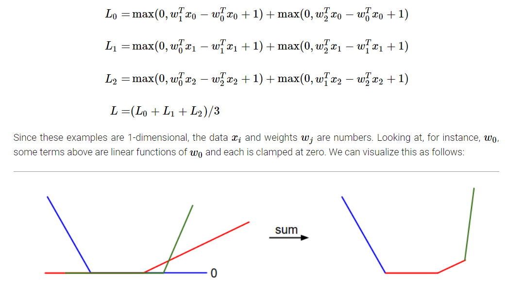
Take loss function of SVM as an example: \[ L_i = \sum_{j\neq y_i}[max(0,w_j^Tx_i-w_{y_i}^Tx_i+\Delta)] \] We can differentiate the function: \[ \Delta_{w_{y_i}}L_i = -(\sum_{j\neq y_i}1_{\{w_j^Tx_i-w_{y_i}^Tx_i+\Delta >0\}}) \\ \Delta_{w_{j}}L_i = 1_{\{w_j^Tx_i-w_{y_i}^Tx_i+\Delta >0\}}x_i \] With grad, we can do Gradient Descent by choosing a suitable step size(or learning rate),
1 | |
However, if the dataset is very big, this can be extremely expensive. So we introduce Mini-batch gradient descent. That means we can only evaluate on a small subset to get a gradient.
The extreme case of this method is the subset has only one image. This process is called Stochastic Gradient Descent(SGD)
Backpropagation, Intuitions
Make good use of chain rule
Ex
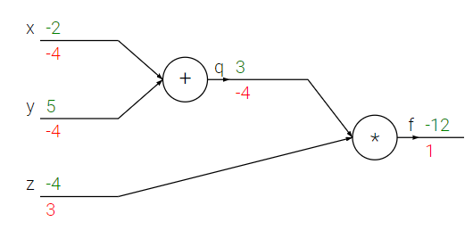
- Add gate
- Max gate
- Multiply gate
Neural Networks Part 1: Setting up the Architecture
input\(\rightarrow\)input\(\cdot\)weight\(\rightarrow\)input\(\cdot\)weight+bias\(\rightarrow\)activate-f(input\(\cdot\)weight+bias)
Ex \[ s=W_2max(0,W_1x)\\ s=W_3max(0,W_2max(0,W_1x)) \]
Single neuron as a linear classifier
- Binary Softmax classifier
- Binary SVM classifier
- Regularization interpretation
Commonly used activation functions
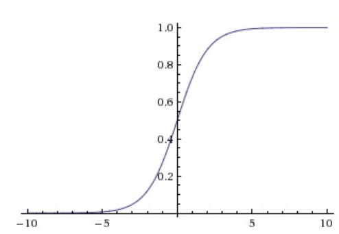
- Sigmoid
\[ \sigma(x)=\frac{1}{1+e^{-x}} \]
Shortcomings:
1. kill gradients
2. not zero-centered
- Tanh
\[ tanh(x)=2\sigma(2x)-1 \]
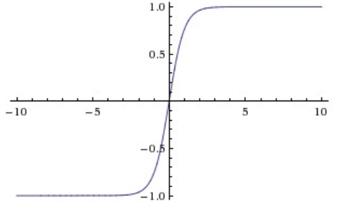
Solve the problem of not zero-centered
- ReLU
\[ f(x)=max(0,x) \]
Advantages: greatly accelerate the convergence of stochastic descent; not so expensive as tanh/sigmoid
Shortcoming: may die when a large gradient flow through a ReLU neuron. May solved by setting a proper learning rate
- Leaky ReLU
\[ f(x)=1_{(x<0)}(\alpha x)+1_{(x>=0)}(x) \]
in which \(\alpha\) is very small like 0.01
- Maxout
\[ max(w_1^Tx+b_1,w_2^Tx+b_2) \]
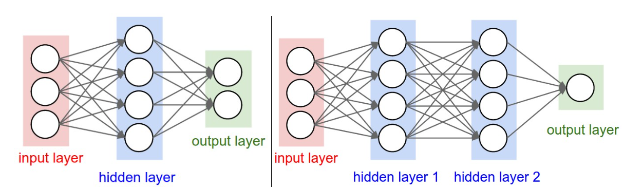
Naming conventions When we talk about N-layer neural network, the input layer is not included in “N”.
Output Layer Unlike other layers, the output layer neurons most commonly do not have an activation function. (while the output layer is used to present scores of every class, it’s easy to understand)
Sizing neural networks Measure the size of neural: number of neurons/number of parameters
Representational power
Surveys has proven that given any continuous function f(x)and some ϵ>0, there exists a Neural Network g(x) with one hidden layer (with a reasonable choice of non-linearity, e.g. sigmoid) such that ∀x,∣f(x)−g(x)∣<ϵ. In other words, the neural network can approximate any continuous function.
Practically, deeper networks can work better than a single-hidden-layer network
For neural network, usually 3-layer networks will be better than 2-layer nets. But more deeper(4,5,6-layer) network rarely helps much more. But for convolutional network , it is different. Depth is a very important factor.
Regularization is very important, which can elite overfitting.
Neural Networks Part 2: Setting up the Data and the Loss
Data Preprocessing
Mean subtraction
code: X-=np.mean(X, axis = 0)
Normalization
code: X/=np.std(X, axis = 0)
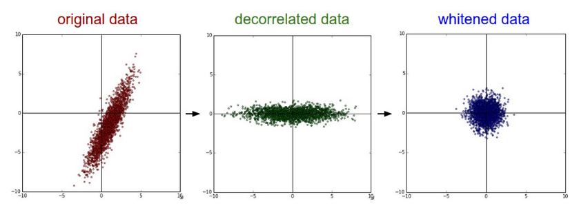
PCA and Whitening
1 | |
compute the SVD factorization of the data covariance matrix:
1 | |
where the columns of
U are the
eigenvectors and
S is a 1-D
array of the singular values. To decorrelate the data, we project the
original (but zero-centered) data into the eigenbasis:
1 | |
dimensionality reduction:
1 | |
For whitening:
1 | |
Common pitfall The mean must be computed only over the training data and then subtracted equally from all splits (train/val/test).
Weight Initialization
Pitfall: all zero initialization That will make every neuron do same thing.
Small random numbers aim: symmetry
breaking. W=0.01*np.random.randn(D, H)
Calibrating the variances with 1/sqrt(n)
W=np.random.randn(n) / sqrt(n) where n is the number of its
inputs
Other: Sparse initialization, Initializing the biases(0), Batch Normalization
Regularization
L2 regularization May the most common. for all \(w\), add \(\frac{1}{2}\lambda w^2\) to the objective.
L1 regularization for each weight \(w\), we add the term \(\lambda |w|\) to the objective.
We can also combine the L1 regularization with the L2 regularization: \(\lambda _1|w|+\lambda_2w^2\), which is called Elastic net regularization.
Max norm constraints Enforce an absolute upper bound on the magnitude of the weight vector.
Dropout keep a neuron active with some probability \(p\) or setting it to zero otherwise
And there are many other methods about regularization. Bias regularization, per-layer regularization…
Loss functions
Let \(f=f(x_i;W)\) to be the activations of the output layer in a Neural Network.
Classification
SVM: \[ L_i=\sum_{j\neq y_i}max(0,f_j-f_{y_i}+1) \]
sometimes use \(max(0,(f_j-f_{y_i}+1)^2)\)
Softmax: \[ L_i=-log(\frac{e^{f_{y_i}}}{\sum_je^{f_j}}) \] Problem: Large number of classes When the set of labels is very large, Softmax becomes very expensive. It may be helpful to use Hierarchical Softmax.
Attribute classification
Both losses above assume that there is a single correct answer \(y_i\). But what if \(y_i\) is a binary vector where every example may or may not have a certain attribute \[ L_i=\sum_jmax(0,1-y_{ij}f_j) \] where \(y_{ij}\) is either +1 or -1
Neural Networks Part 3: Learning and Evaluation
Talking about learning process.
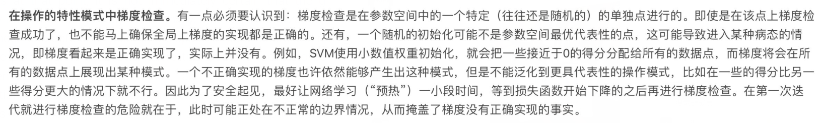
Gradient Checks
\[ \frac{df(x)}{dx}=\frac{f(x+h)-f(x-h)}{2h} \]
In order to compare the numerical gradient \(f_n'\) and analytic gradient \(f_a'\), we can use relative error: \[ \frac{|f_a'-f_b'|}{max(|f_a'|,|f_n'|)} \] In practive:
- relative error >\(1e-2\): probably wrong
- 1e-2>relative error>1e-4: uncomfortable…
- 1e-4>relative error: OK…but without kinks(e.g. tanh and softmax), to high.
- 1e-7>relative error: happy
should use double precision
if jump kinks, may not be exact
In order to avoid above problems:
- Use only few datapoints
- be careful with h
Don’t let the regularization overwhelm the data
Remember to turn off dropout/augmentations
Before learning: sanity checks Tips/Tricks
- Trace loss function
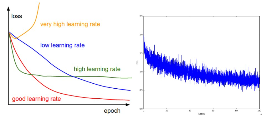
The right picture may mean the data is so small
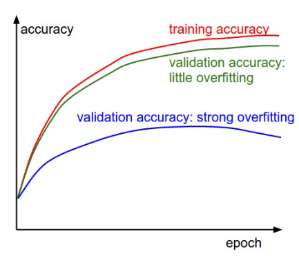
- Trace train/val accuracy
- Ratio of weights: updates
Ex
1 | |
Activation / Gradient distributions per layer
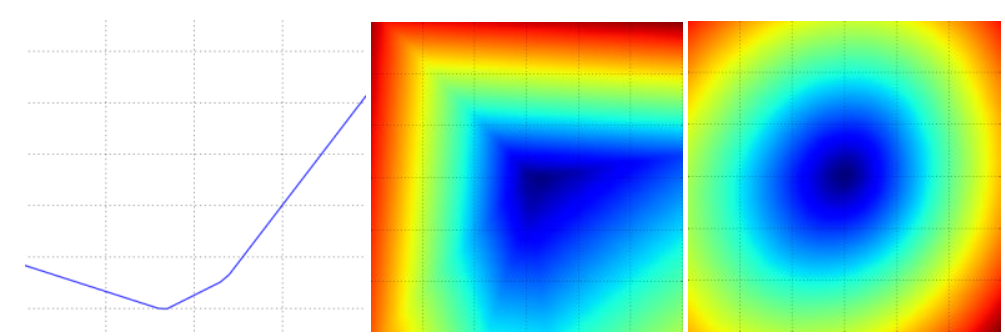
First-layer Visualizations
Ex
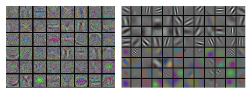
Left: many noise. may in trouble. Right: Nice, smooth
Parameter updates
First-order(SGD), momentum, Nesterov momentum
- Vanilla update
1 | |
- Momentum update
1 | |
mu can be seen as the coefficient of friction in physics. (typical 0.9)
- Nesterov Momentum
1 | |
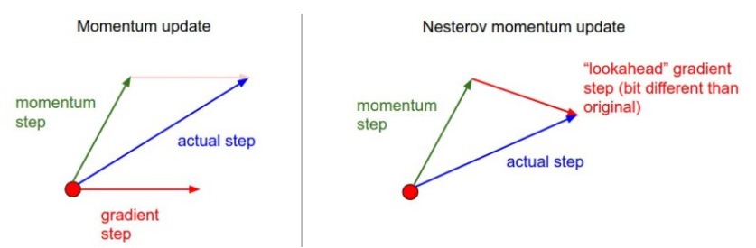
In practice, people like to rename \(x\_head\) as \(x\) :
1 | |
Annealing the learning rate
If the learning rate is too high, the system contains too much kinetic energy, unable to settle down into deeper, but narrower parts of the loss function.
Normally, there are three methods to decay the learning rate:
- Step decay Reduce the learning rate every few epochs.
- Exponential decay In math: \(\alpha = \alpha_0e^{-kt}\) in which \(\alpha_0,k\) are hyperparameters and \(t\) is the iteration number.
- 1/t decay In math: \(\alpha = \alpha _0/(1+kt)\) in which \(\alpha_0,k\) are hyperparameters and \(t\) is the iteration number
In practice, we find that the step decay is slightly preferable because the hyperparameters it involves
Second order methods
Basing on Newton’s method: \[ x\leftarrow x-[Hf(x)]^{-1}\nabla f(x) \] Multiplying by the inverse Hessian leads the optimization to take more aggressive steps in directions of shallow curvature and shorter steps in directions of steep curvature
However, because of the expensive cost of calculating the Hessian matrix, this method is impractical.
Per-parameter adaptive learning rate methods
Adagrad is an adaptive learning rate method originally proposed by Duchi et al.
1 | |
eps: 1e-4~1e-8
shortcoming: the monotonic learning rate usually proves too aggressive and stops learning too early
RMSprop slide 29 of Lecture 6 of Geoff Hinton’s Coursera class: reduce Adagrad’s aggressive
1 | |
in which decay_rate is a hyperparameter: 0.9, 0.99,
0.999
Adam a recently proposed update looks a bit like RMSprop with momentum
simplified:
1 | |
recommend: eps = 1e-8, beta1 = 0.9,
beta2 = 0.999
With the bias correction mechanism, the update looks as follows:
1 | |
Hyperparameter optimization
The most common hyperparameters in context of Neural Networks include:
- the initial learning rate
- learning rate decay schedule(such as the decay constant)
- regularization strength(L2 penalty, dropout strength)
Implementation make a worker and master
Prefer one validation fold to cross-validation a single validation set of respectable size substantially simplifies the code base, without the need for cross-validation with multiple folds
Hyperparameter ranges
learning_rate = 10 ** uniform(-6, 1)
Prefer random search to grid search can be easily understand through following image:
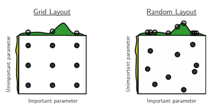
Careful with best values on border if we find that the results is on the border, we may set a bad range and miss the true best result.
Stage your search from coarse to fine
Bayesian Hyperparameter Optimization Spearmint, SMAC, and Hyperopt. However, in practical settings with ConvNets it is still relatively difficult to beat random search in a carefully-chosen intervals.
Evaluation
Model Ensembles
A reliable way to improve the performance of Neural Networks by a few percent: train multiple independent models, and at test time average their predictions.
The number of models \(\uparrow\) performance \(\uparrow\) the variety of models \(\uparrow\) performance \(\uparrow\)
Some approaches to forming an ensemble
- Same model, different initializations
Use cross-validation to determine the best hyperparameters, then train multiple models with the best set of hyperparameters but with different random initialization.
shortcoming: variety is only due to iitialization
Top models discovered during cross-validation
Use cross-validation to determine the best hyperparameters, then pick the top few (e.g. 10) models to form the ensemble.
shortcoming: may include suboptimal models
- Different checkpoints of a single model
Taking different checkpoints of a single network over time is training is very expensive
shortcoming: lack of variety
advantage: very cheap
- Running average of parameters during training
Shortcoming of model ensembles: take longer to evaluate on test example.
A good idea: “distill” a good ensemble back to a single model by incorporating the ensemble log likelihoods into a modified objective.
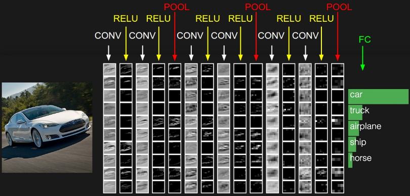
Convolutional Neural Networks
Convolutional Neural Networks: Architectures, Convolution / Pooling Layers
CNN base on an assumption that the inputs are images.
Layers used to build ConvNets
Convolutional Layer, Pooling Layer, Fully-Connected Layer
Convolutional Layer
filter with size like \(5\times 5\times 3\)
During the forward pass, we slide (more precisely, convolve) each filter across the width and height of the input volume and compute dot products between the entries of the filter and the input at any position
\(\rightarrow\) produce a separate 2-dimensional activation map
The spatial extent of this connectivity: a hyperparameter called the receptive field
Depth, Stride, Zero-padding
Depth: depend on the number of filter. Called “deep column” or “fiber”
Stride: the number of pixel the filter will move when we slide it
Zero-padding: pad the input volume with zeros around the border
In math. the input volume size :\(W\), the receptive size of the Conv Layer neurons: \(F\), the stride with which they are applied: \(S\), the amount of zero padding used: \(P\)
then the output: \((W-F+2P)/S+1\)
Summary
Accept size: \(W_1\times H_1\times D_1\)
Require:
- number of filters \(K\)
- spatial extent \(F\)
- stride \(S\)
- the amount of zero padding \(P\)
Produce size: \(W_2 \times H_2 \times D_2\)
- \(W_2=(W_1-F+2P)/S+1\)
- \(H_2=(H_1-F+2P)/S+1\)
- \(D_2=K\)
common set: \(F=3, S=1, P=1\)
Backpropagation The backward pass for a convolution operation (for both the data and the weights) is also a convolution (but with spatially-flipped filters).
\(1\times 1\) convolution note that we have 3 channels. so it’s not meaningless
Dilated convolutions have filters that have spaces between each cell, called dilation.
##### Pooling layer
Common: Max
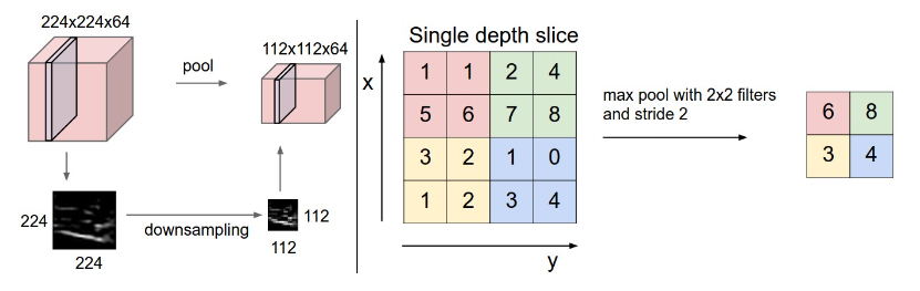
Accept size \(W_1\times H_1\times D_1\)
Hyperparameters
- spatial extent \(F\)
- stride \(S\)
Produce size \(W_2\times H_2\times D_2\)
- \(W_2=(W_1-F)/S+1\)
- \(H_2=(H_1-F)/S+1\)
- \(D_2=D_1\)
Common: \(F=3, S=2\) more commonly \(F=2, S=2\)
Normalization Layer
These layers have since fallen out of favor because in practice their contribution has been shown to be minimal, if any. For various types of normalizations, see the discussion in Alex Krizhevsky’s cuda-convnet library API.
Fully-connected layer
Just like Neural Network section
Converting Fully Connected layers to CONV layers
Each of these conversions could in practice involve manipulating (e.g. reshaping) the weight matrix \(W\) in each FC layer into CONV layer filters. It turns out that this conversion allows us to “slide” the original ConvNet very efficiently across many spatial positions in a larger image, in a single forward pass.
ConvNet Architectures
The most common pattern:
1 | |
N >= 0 (and usually N <= 3),
M >= 0, K >= 0 (and usually
K < 3).
INPUT -> FC, implements a linear classifier.INPUT -> CONV -> RELU -> FCINPUT -> [CONV -> RELU -> POOL]*2 -> FC -> RELU -> FC. Here we see that there is a single CONV layer between every POOL layer.INPUT -> [CONV -> RELU -> CONV -> RELU -> POOL]*3 -> [FC -> RELU]*2 -> FCHere we see two CONV layers stacked before every POOL layer.
Prefer a stack of small filter CONV to one large receptive field CONV layer.
Layer Sizing Patterns
- Input Layer
Should be divisible by 2 many times.
Ex. 32 (e.g. CIFAR-10), 64, 96 (e.g. STL-10), or 224 (e.g. common ImageNet ConvNets), 384, and 512.
- Conv Layer
3x3 or 5x5 Step \(S=1\), zero
- Pool Layer
2x2 , stride = 2(sometimes 3x3, stride = 2)
Use stride of 1 in CONV:
- Smaller strides work better in practice.
- Allows us to leave all spatial down-sampling to the POOL layers, with the CONV layers only transforming the input volume depth-wise.
Use padding:
If the CONV layers were to not zero-pad the inputs and only perform valid convolutions, then the size of the volumes would reduce by a small amount after each CONV, and the information at the borders would be “washed away” too quickly.
Compromising based on memory constrains:
people prefer to make the compromise at only the first CONV layer of the network. For example, one compromise might be to use a first CONV layer with filter sizes of 7x7 and stride of 2 (as seen in a ZF net). As another example, an AlexNet uses filter sizes of 11x11 and stride of 4.
Case Studies
- LeNet
- AlexNet
- ZF Net
- GoogleNet
- VGGNet
- ResNet
VGG:
1 | |
Computational Considerations
There are three major sources of memory to keep track of:
From the intermediate volume sizes
From the parameter sizes
Every ConvNet implementation has to maintain miscellaneous memory, such as the image data batches, perhaps their augmented versions, etc.
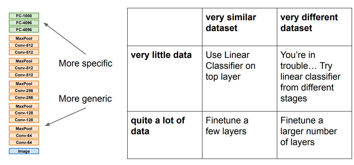
Transfer Learning and Fine-tuning Convolutional Neural Networks
Transfer Learning